Table of Contents

What Is Fractal Geometry?

Fractal geometry is a branch of mathematics that studies shapes and structures exhibiting self-similarity — patterns that repeat at every level of magnification. Coined by mathematician Benoit Mandelbrot in 1975, the term “fractal” comes from the Latin word fractus, meaning broken or fragmented. Unlike classical Euclidean geometry, which deals with smooth lines and perfect circles, fractal geometry describes the rough, irregular shapes that actually dominate the natural world.

Why Regular Geometry Falls Short

Here’s something that probably never bothered you until right now: classical geometry can’t describe a cloud. Or a mountain. Or the branching pattern of your lungs.

Euclid gave us beautiful tools — circles, triangles, rectangles — and for two thousand years, those shapes were the language of mathematics. Buildings, bridges, and blueprints all speak Euclidean. But step outside, and almost nothing in nature fits those tidy categories.

A coastline isn’t a straight line. A tree isn’t a cylinder topped with a sphere. Your circulatory system isn’t a series of tubes in decreasing size (well, it sort of is — but describing it with classical geometry would take forever and miss the pattern entirely).

Mandelbrot noticed this gap in the 1960s and 1970s while working at IBM. He was studying cotton price fluctuations, and the data looked… the same, no matter what time scale he examined. Daily price changes had the same statistical pattern as monthly and yearly ones. That self-similarity across scales — the mathematical signature of a fractal — kept showing up everywhere he looked.

His 1982 book, The Fractal Geometry of Nature, essentially argued: the geometry we’ve been using for millennia is the wrong language for describing most of the physical world. He was right.

Self-Similarity: The Core Idea

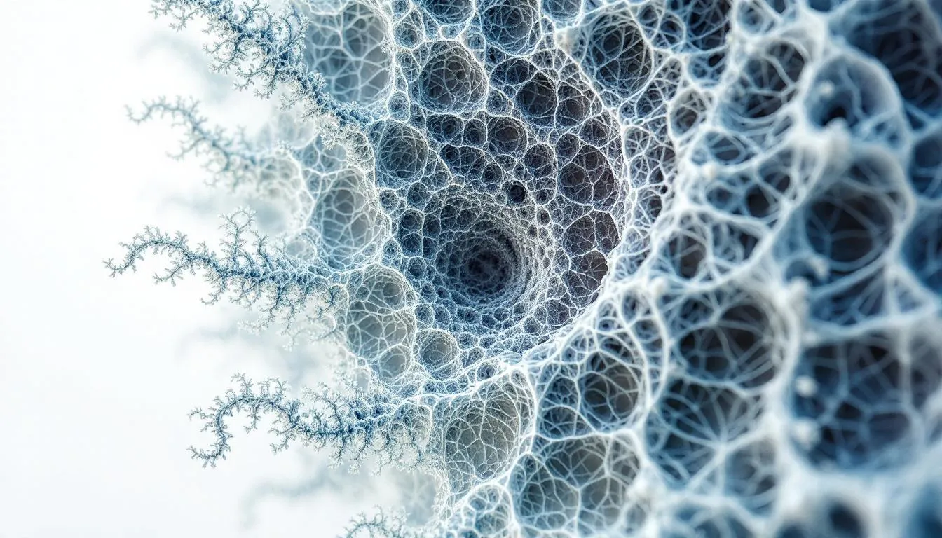
The defining feature of a fractal is self-similarity. Zoom in on part of a fractal, and you see a smaller copy of the whole thing. Zoom in further — same pattern. Again and again, potentially forever.

There are different flavors of this:

Exact self-similarity means the zoomed-in portion is a perfect, identical copy of the whole. Mathematical fractals like the Sierpinski triangle and Koch snowflake have this property. They’re constructed by repeating simple rules infinitely.

Quasi self-similarity means the zoomed-in portions are approximately (but not perfectly) similar to the whole. The Mandelbrot set does this — as you zoom in, you find small copies of the overall shape, but each copy has unique, new details around it.

Statistical self-similarity means the statistical properties (not the exact shapes) repeat across scales. This is what you find in nature. A small section of coastline has similar roughness statistics to a large section, even though they’re not identical shapes.

That third type is the one that matters most in real-world applications. Nature doesn’t produce perfect mathematical objects, but it produces patterns that fractal mathematics can describe with stunning accuracy.

The Famous Fractals You Should Know

The Mandelbrot Set

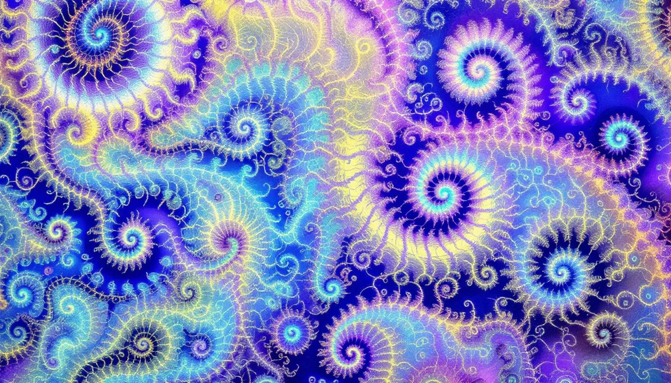
If you’ve ever seen a fractal image — those psychedelic, infinitely swirling shapes — you’ve probably seen the Mandelbrot set. It’s generated by an absurdly simple equation: z = z² + c, where z and c are complex numbers.

For each point c on the complex plane, you iterate the equation starting from z = 0. If the sequence stays bounded (doesn’t fly off to infinity), that point is in the Mandelbrot set. Color the bounded points black and the unbounded points by how fast they escape, and you get the most famous image in mathematics.

The astonishing part? This simple equation produces infinite complexity. You can zoom into the boundary of the Mandelbrot set forever and keep finding new patterns — spirals, seahorse tails, miniature copies of the whole set, structures that look like nothing you’ve named before. Mathematicians have been exploring it since the 1980s and haven’t exhausted its surprises.

The Mandelbrot set lives on the boundary between order and chaos. Points clearly inside are stable. Points clearly outside diverge quickly. The boundary itself — that’s where all the action is.

The Koch Snowflake

Start with an equilateral triangle. Divide each side into three equal parts. Replace the middle third with two sides of a smaller equilateral triangle (pointing outward). Repeat for every line segment, forever.

The Koch snowflake has some mind-bending properties. Its area is finite — specifically, 8/5 of the original triangle’s area. But its perimeter is infinite. An enclosed, finite shape with an infinitely long border. That’s what fractals do to your intuitions about geometry.

The Sierpinski Triangle

Take an equilateral triangle. Remove the middle triangle (the one formed by connecting the midpoints of each side). Now you have three smaller triangles. Remove the middle of each. Repeat infinitely.

What’s left? A shape with zero area but infinite perimeter. It’s technically dust — an infinite collection of points with no solid surface. Yet the pattern is instantly recognizable and strangely beautiful. The Sierpinski triangle has a fractal dimension of about 1.585 — more than a line (dimension 1) but less than a filled triangle (dimension 2).

Julia Sets

Closely related to the Mandelbrot set, Julia sets use the same equation (z = z² + c) but hold c constant and vary the starting point z. Each value of c produces a different Julia set. Some are connected, lush, and swirling. Others are totally disconnected — fractal dust scattered across the plane.

Here’s the beautiful connection: the Mandelbrot set is essentially a map of all Julia sets. If c is inside the Mandelbrot set, the corresponding Julia set is connected. If c is outside, the Julia set is disconnected. The Mandelbrot set is a directory of an infinite family of fractals.

Fractal Dimension: When 1, 2, and 3 Aren’t Enough

In regular geometry, dimension is straightforward. A point is 0-dimensional. A line is 1-dimensional. A plane is 2-dimensional. A cube is 3-dimensional. Always whole numbers.

Fractals break this rule. Their dimensions are typically non-integers — fractions that fall between the familiar whole numbers.

The intuition goes like this: a fractal line (like a coastline) is more than a 1D line because it wiggles and fills more space than a straight line would. But it’s less than a 2D plane because it doesn’t fill a solid area. So its dimension falls somewhere between 1 and 2.

The most common way to calculate fractal dimension is the box-counting method. Cover the fractal with boxes of side length s, and count how many boxes (N) you need. As you shrink s, N grows. The fractal dimension D satisfies the relationship N ~ s^(-D). For a straight line, D = 1. For a filled square, D = 2. For the Koch snowflake, D ≈ 1.26. For the coastline of Great Britain, D ≈ 1.25.

This matters practically, not just theoretically. Fractal dimension gives scientists a single number to characterize the roughness or complexity of natural surfaces, boundaries, and patterns. The fractal dimension of lung tissue changes with disease. The fractal dimension of a city’s street network tells you about its growth patterns. The fractal dimension of a stock market time series signals volatility.

Fractals in Nature: Everywhere You Look

Once you understand fractals, you start seeing them everywhere. And frankly, it’s a little unsettling how universal these patterns are.

Coastlines and the Measurement Problem

Mandelbrot’s famous 1967 paper asked: “How long is the coast of Britain?” The answer, surprisingly, is that it depends on your ruler. Measure with a 200 km ruler, you get one answer. Use a 50 km ruler, and the coast is longer — the shorter ruler captures more of the jagged inlets and bays. Use a 1 km ruler, even longer. A 1-meter ruler, longer still.

The coastline doesn’t converge to a fixed length as your ruler shrinks. It keeps getting longer. This is the fractal nature of coastlines — roughness at every scale. The rate at which the measured length increases as the ruler shrinks gives you the fractal dimension.

Trees and Branching

Look at a tree. The trunk splits into major branches. Those branches split into smaller branches. Those split into twigs. Twigs split into smaller twigs. The branching pattern is self-similar — each fork looks like a miniature version of the whole tree.

This isn’t coincidence. It’s biology optimizing for resource distribution. A tree needs to deliver water and nutrients to every leaf while minimizing the total “plumbing” needed. Fractal branching turns out to be an incredibly efficient solution to this distribution problem. Your circulatory system uses the same strategy — arteries branch into arterioles, then capillaries, in a fractal pattern that delivers blood to every cell.

Rivers and Drainage

River systems form fractal patterns. Small streams feed into larger streams, which feed into rivers, which feed into major rivers. Viewed from above, a river drainage basin looks startlingly like a tree — or like your circulatory system. The fractal dimension of river networks is remarkably consistent worldwide, typically around 1.8 to 1.9.

Mountains and Terrain

Mountain ranges aren’t smooth. They’re rough at every scale — from the shape of entire ranges down to individual boulders and rocks. This fractal roughness is why computer graphics artists use fractal algorithms to generate realistic terrain. You can’t tell the difference between a fractal mountain and a photograph of a real one.

Clouds and Weather

Clouds are fractal. Their edges are rough and self-similar across scales. More importantly, weather patterns themselves show fractal-like behavior — the same kinds of turbulent structures appear at scales from centimeters to hundreds of kilometers. This connects to chaos theory, where small changes in initial conditions produce dramatically different outcomes, creating the unpredictability that makes weather forecasting so difficult beyond about 10 days.

The Math Behind the Beauty

Iterated Function Systems (IFS)

Many fractals can be described as iterated function systems — collections of contraction mappings applied repeatedly. Each mapping takes the current shape and creates a smaller, transformed copy. Apply all the mappings, and you get the next iteration. Repeat infinitely, and you reach the fractal.

The Sierpinski triangle, for example, can be generated by three affine transformations, each shrinking the shape by half and moving it to one corner. The magic of IFS is that vastly different-looking fractals can be encoded in just a few numbers — the parameters of the transformations.

This is the basis of fractal image compression. Michael Barnsley developed algorithms in the late 1980s that compress images by finding IFS codes that approximate them. The compressed file stores just the transformations, not the pixels. Decompressing means iterating those transformations until the image emerges. For certain types of images (especially natural scenes), fractal compression achieves remarkable compression ratios.

L-Systems and Plant Growth

Aristid Lindenmayer invented L-systems in 1968 to model plant growth. An L-system is a string-rewriting grammar — you start with a seed string and apply replacement rules repeatedly. Map the resulting string to drawing instructions (move forward, turn left, turn right, push position, pop position), and you get astonishingly realistic plant structures.

A simple L-system with two rules can generate a convincing fern. A slightly more complex one creates a realistic tree. Botanists use L-systems to study how genetic instructions produce the fractal branching patterns we see in real plants. Algorithms based on L-systems generate the vegetation in video games and movies.

Strange Attractors and Chaos

Fractal geometry and chaos theory are deeply intertwined. When you plot the long-term behavior of a chaotic system — say, the Lorenz equations that model atmospheric convection — the trajectories trace out a fractal shape called a strange attractor.

The Lorenz attractor looks like a butterfly’s wings. It has a fractal dimension of about 2.06. The system never repeats exactly, but it stays on this fractal structure forever. This is chaos in action: deterministic (the equations have no randomness) but unpredictable (tiny differences in starting conditions lead to completely different paths on the attractor).

Edward Lorenz discovered this in 1963 while modeling weather on an early computer. He rounded an input from 0.506127 to 0.506, and the simulation diverged completely. That sensitivity — the famous “butterfly effect” — is a hallmark of chaotic systems, and the strange attractors they produce are always fractal.

Fractals in Technology

Computer Graphics and Terrain Generation

Before fractals, generating realistic natural scenes in computer graphics was almost impossible. Smooth mathematical surfaces look artificial. Fractal algorithms changed everything.

The midpoint displacement method generates fractal terrain by recursively subdividing a surface and randomly displacing the midpoints. Control the displacement amount, and you control the roughness — smooth rolling hills or jagged mountains. Pixar, Industrial Light & Magic, and every major effects studio uses fractal techniques (among others) to create landscapes, clouds, fire, and water.

The 1982 film Star Trek II: The Wrath of Khan featured the “Genesis Effect” — one of the first uses of fractal field generation in film. Loren Carpenter at Lucasfilm created it using fractal subdivision, and it stunned audiences and filmmakers alike.

Antenna Design

Here’s a practical application that affects your daily life: the antenna in your phone is probably fractal-shaped. A fractal antenna packs more electrical length into a smaller physical space because the self-similar shape creates resonance at multiple frequencies simultaneously.

Traditional antennas are tuned to specific frequencies based on their length. A fractal antenna, with its many length scales, can operate across a broader range of frequencies. This is why your phone can handle cellular, Wi-Fi, Bluetooth, and GPS with a single small antenna. Nathan Cohen developed the first fractal antennas in 1988, and they’re now standard in virtually all wireless devices.

Medical Imaging and Diagnosis

Your body is full of fractal structures — blood vessels, neurons, lung airways, intestinal villi. When disease disrupts these patterns, the fractal dimension changes. Researchers use fractal analysis to detect:

Cancer: Tumor blood vessel networks have different fractal dimensions than healthy vasculature. Some studies show fractal analysis of mammograms can improve cancer detection rates.
Retinal disease: The branching pattern of retinal blood vessels is fractal, and changes in fractal dimension correlate with diabetic retinopathy and glaucoma.
Heart disease: Heart rate variability is fractal in healthy hearts. Loss of fractal complexity in the heartbeat signal predicts cardiac problems.
Osteoporosis: Bone trabecular structure is fractal. Anatomy researchers measure its fractal dimension to assess bone health.

Signal and Image Processing

Fractal mathematics shows up in digital signal processing and data analysis. Many natural signals — seismic data, financial time series, network traffic, audio recordings — have fractal properties. Their power spectra follow power laws (the signature of self-similarity), and fractal-based methods often outperform traditional analysis for these signals.

Wavelet transforms, now essential in signal processing and image compression (they’re part of JPEG 2000), have deep connections to fractal theory. Both deal with information at multiple scales simultaneously.

Fractals and Finance

Mandelbrot himself spent considerable time applying fractal geometry to financial markets. His 1963 paper on cotton prices showed that price changes don’t follow the normal (Gaussian) distribution that most financial models assumed. Instead, they follow a distribution with “fat tails” — extreme events happen far more often than the bell curve predicts.

This matters enormously. The 2008 financial crisis involved events that standard models rated as essentially impossible — once-in-a-billion-years unlikely. Fractal models, which account for self-similar volatility clustering, would have assigned those events much higher probabilities.

Financial time series are statistically self-similar. Zoom into a price chart without labels, and you genuinely can’t tell if you’re looking at five minutes, five days, or five years of data. The patterns of volatility clustering, trend following, and mean reversion repeat across time scales. This is exactly what fractal geometry describes.

Mandelbrot’s “multifractal model of asset returns” remains an active research area. It hasn’t replaced standard models in practice (partly because it’s mathematically harder to work with), but the insight — that financial markets are fractal, not Gaussian — has fundamentally changed how quantitative researchers think about risk.

How to Generate Fractals Yourself

You don’t need advanced mathematics to create fractals. The basic algorithms are surprisingly accessible.

The Chaos Game

Here’s possibly the simplest fractal generator ever devised. Place three points as the vertices of a triangle. Pick any starting point. Now, repeatedly:

Randomly choose one of the three vertices
Move halfway toward it
Plot the new point
Repeat

After thousands of iterations, the Sierpinski triangle emerges from what seems like random chaos. This works because the random process is exploring an IFS — the three “move halfway” rules are exactly the contraction mappings that define the Sierpinski triangle.

Escape-Time Algorithms

The Mandelbrot set and Julia sets use escape-time algorithms. For each point in the complex plane, iterate z = z² + c and check whether the sequence escapes (|z| > 2) or stays bounded. Color based on how many iterations it takes to escape. The boundary between escaping and bounded points is where the fractal structure lives.

Modern GPU-accelerated renderers can generate Mandelbrot zooms in real time, diving deeper and deeper into the infinite fractal structure. Some of the deepest zooms calculated reach magnification factors of 10^2000 — a number so large it makes the size of the observable universe look like a rounding error.

Random Fractal Landscapes

Fractal terrain generation using the diamond-square algorithm is another accessible project. Start with a grid of corner heights. For each square, set the center height to the average of the corners plus a random offset. For each diamond, set the center to the average of the diamond corners plus a random offset. Reduce the random offset at each scale. The result: realistic-looking computer graphics terrain from pure mathematics.

The Philosophy of Fractals

Fractals raise genuine philosophical questions about the nature of mathematics and reality.

Euclidean geometry was considered the “language of nature” for millennia. It turns out nature speaks a different language — one of recursion, iteration, and self-similarity. The smooth, regular shapes of Euclid are human abstractions. The rough, fractal shapes Mandelbrot described are what actually exists.

This raises a question: are fractals discovered or invented? The Mandelbrot set exists as a mathematical object regardless of whether anyone computes it. Its infinite complexity emerges from one simple equation. Some mathematicians argue this makes it more “real” than physical objects — it exists in a platonic area of mathematical truth, and we merely explore it.

Others counter that fractals in nature are approximations — statistical, not exact. A real coastline doesn’t have infinite detail. A real tree doesn’t branch forever. The mathematical idealization and the physical reality are related but distinct.

Either way, fractal geometry changed how we see the world. Before Mandelbrot, roughness and irregularity were seen as noise — imperfections overlaid on some underlying smooth reality. Fractal geometry reframes them as the primary signal. The roughness is the geometry. The irregularity is the pattern. Understanding that shift is understanding fractal geometry.

What Fractal Geometry Means for Other Fields

Fractal thinking has spread far beyond mathematics. In biology, researchers describe the fractal architecture of ecosystems, from individual organisms to entire biomes. In data science, fractal analysis characterizes everything from internet traffic to earthquake patterns. In architecture, designers use fractal scaling to create buildings that feel natural and harmonious — because, some researchers argue, our visual system is tuned to prefer fractal patterns with dimensions around 1.3 to 1.5.

The deeper insight of fractal geometry isn’t any particular formula or shape. It’s the recognition that complexity can arise from simplicity through repetition. A few simple rules, applied recursively, generate infinite variety. That principle shows up everywhere — in cellular automata, in genetic codes, in the structure of the universe itself.

Mandelbrot once said, “Clouds are not spheres, mountains are not cones, coastlines are not circles, and bark is not smooth, nor does lightning travel in a straight line.” Fractal geometry is the mathematics that finally takes those messy, beautiful realities seriously.

Key Takeaways

Fractal geometry studies self-similar shapes — patterns that repeat at every scale. Developed primarily by Benoit Mandelbrot in the 1970s and 1980s, it provides mathematical tools to describe the roughness and irregularity found throughout nature, from coastlines and mountains to blood vessels and galaxies.

Fractals have non-integer dimensions, challenging our basic intuitions about space. They’re generated by simple rules applied recursively, producing infinite complexity from finite instructions. And they’ve found practical applications in antenna design, medical imaging, computer graphics, financial modeling, and signal processing.

More than a branch of mathematics, fractal geometry is a way of seeing. It reveals the hidden order in apparent chaos and the infinite detail lurking in the everyday shapes around you.

Frequently Asked Questions

What is the simplest example of a fractal?

The Sierpinski triangle is one of the simplest fractals. Start with an equilateral triangle, remove the middle triangle, and repeat for each remaining triangle forever. The resulting shape has infinite detail and zero area — a classic fractal.

Are fractals actually infinite?

Mathematically, yes — a true fractal has infinite detail at every scale. In nature, fractal-like patterns exist across many scales but eventually stop. A coastline looks jagged at 1,000 km and 1 km, but at the atomic level, the pattern breaks down.

How are fractals used in technology today?

Fractals are used in image compression (fractal compression algorithms), antenna design (fractal antennas fit more length in less space), computer graphics for realistic terrain and clouds, signal processing, and even medical imaging to detect irregular tissue growth.

What is fractal dimension?

Fractal dimension measures how a fractal's detail changes with scale. Unlike regular shapes (a line is 1D, a square is 2D), fractals have non-integer dimensions. The coastline of Britain, for example, has a fractal dimension of about 1.25 — more than a line but less than a plane.